MATLAB
MATLAB for MATH241H - Section 0301 - Fall 2017
MATLAB Project 1 Due: W 10/4
The following material has been adapted and copied with permission from material created by Justin Wyss-Gallifent.
The basic format of this Guide/Project is that you will sit down with this guide open and Matlab running and try things as you go.
The Guide/Project has various Tasks interspersed within. The project involves creating a script m-file and put the tasks in order into that file, then publishing that file.
Running Matlab
There are several ways to access Matlab on campus:
- You can dowload the latest version as a student for free from UMD's terpware website
- Through one of the many computer lab locations around campus with access to MATLAB. For instance, the math OWL Lab in MATH 0203.
- Through the Engineering department's Virtual lab
Okay, I’m running Matlab, now what?
When you run Matlab you will see a bunch of windows. The important one will have a prompt in it which looks like <<. This is where we will tell Matlab what to do.
Go into this window and type 2+3. You will see:
2+3ans =
5Oh yeah, you know Matlab! Let’s do something more relevant to calculus like take a derivative. Before we do that it’s important to note that Matlab works a lot with what are called symbolic expressions. If we want to take a derivative we use the diff command. It’s tempting to do diff(x^2) but produces an error. Try it and see!
Why does it error? The reason is that Matlab doesn’t know what x is and we must tell it that x is a symbol to work with. We do so with the syms command. So we can do the following two commands.
The first line tells Matlab that x is symbolic and will be symbolic until we tell it otherwise.
syms x
diff(x^2)
ans =
2*xEat your heart out Newton and Leibniz! Here’s an even uglier derivative. Keep in mind that we don’t need a syms x now because x is still symbolic and will remain so from our previous declaration. Notice something important - that multiplication in Matlab always needs a *. Leaving this out will give an error.
diff(2*x^2*sin(x)/cos(x))ans =
2*x^2 + (2*x^2*sin(x)^2)/cos(x)^2 + (4*x*sin(x))/cos(x)Oh boy, that’s pretty messy. Can we simplify that at all? Indeed we can. We can wrap it in the Matlab command simplify as follows:
simplify(2*diff(x^2*sin(x)/cos(x)))ans =
(2*x*(x + sin(2*x)))/cos(x)^2Precalculus
Here are some precalculus things done in Matlab.
Solving and equation
Here we solve the equation $x^2 + x -1 = 0$
solve(x^2+x-1)ans =
-5^(1/2)/2 - 1/2
5^(1/2)/2 - 1/2Note the the expression given to solve assumes that it is looking for zeros of the symbolic expression given to it. We can tell it to equal something else too. Note the == we use. In some cases Matlab will accept a single equals sign but Matlab is currently undergoing changes to bring it in line with most programming languages. Typically single = are used for assigning variables whereas double == are used to check for equality. Solving an equation really means checking when two things are the same,
hence ==.
solve(x^2+x-1 == 1)ans =
-2
1Substitute a value into a symbolic expression
Here we tell Matlab to put -1 in place of x. The reason it knows to put it in place of x is that x is the only variable.
subs(x^3+4/x+1,-1)ans =
-4If you have multiple variables, then you should tell it which variable to substitute for. If you don’t then it will make assumptions and those assumptions may confused you. So here I’ll redeclare our variables just for clarity and then substitute for y:
syms x y
subs(x^2+y^2+x+y,y,2)
ans =
x^2 + x + 6Plot a function
There are many ways to plot in Matlab but the easiest way has the name fplot. When you run it you will get a new window which will pop up. In this tutorial the picture is embedded in the text. The fplot command tries to make reasonable choices as to the amount of the graph to show. Also it does not draw axes, instead it puts the graph in a box. I find that annoying but maybe you like boxes and other rectangular shapes. Honestly the reason Matlab does this is so the axes stay out of the way and you can see what’s going on.
fplot(x+3*sin(x))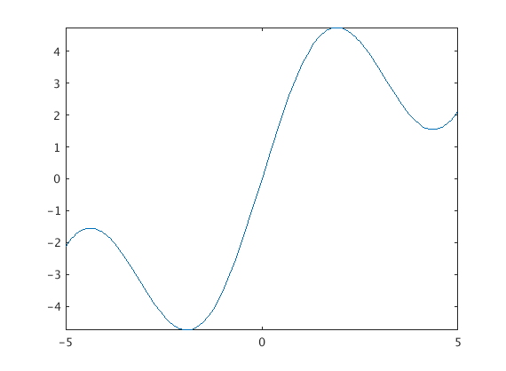
If you want to give it a specific domain of x-values you can do that too:
fplot(x+3*sin(x),[-3,3])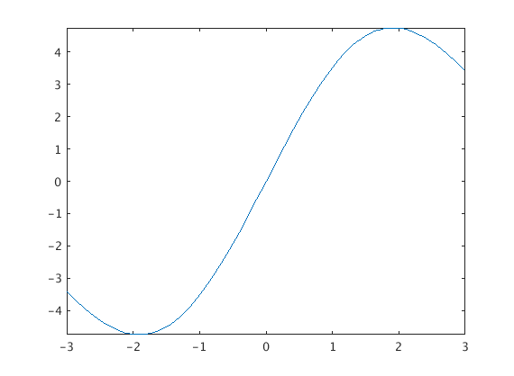
Calculus I
We can also do some basic calculus.
Take a derivative and substitute
The following code takes the derivative of $x^3$ and evaluates is at $x=3$.
subs(diff(x^3),x,3)ans =
27Notice that subs is wrapped around diff. If we wrap diff around subs look at what happens and think about why. Do you know why?
diff(subs(x^3,x,3))ans =
0Finding an indefinite integral
Notice that Matlab, like many careless students, never puts a $+c$ in its indefinite integrals. Grrr.
int(x*sin(x))ans =
sin(x) - x*cos(x)Finding a definite integral
We can also find indefinite integrals.
int(x*sin(x),0,pi/6)ans =
1/2 - (pi*3^(1/2))/12Calculus II
Plotting a parametric curve
Plot the parametric curve $x = \cos{t}$ and $y = \sin{t}$ for $0 \leq t \leq \pi$. Note that this also a Calculus III problem if we think of this as plotting the vector-valued function given by $\mathbf{r}(t) = \cos{t}\,\mathbf{i} + \sin{t}\,\mathbf{j}$. Notice also the new symbolic variable t is declared.
syms t
fplot(cos(t),sin(t),[0,pi])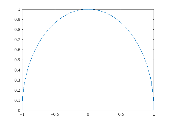
Calculus III
Vectors
Vectors in Matlab are treated like in linear algebra so this may be new to you. The vector $2\mathbf{i} + 3\mathbf{j} + 7\mathbf{k}$ can be entered either as a horizontal vector or a vertical vector. Whatever you choose to use, be consistent. I will use horizontal vectors in this guide because that’s how we think of them in Math 241, except with $\mathbf{i}$, $\mathbf{j}$ and $\mathbf{k}$.
As a horizontal vector (like I’ll do) we use spaces or commas to separate values.
u=[2,3,7]u =
2 3 7We can put variables inside vectors too for vector-valued functions and then take derivatives:
a=[t^2,1/t,2*t]
diff(a)
int(a,1,3)a =
[ t^2, 1/t, 2*t]
ans =
[ 2*t, -1/t^2, 2]
ans =
[ 26/3, log(3), 8]Combinations of Vectors
Here are various combinations of vectors. Notice also here the semicolons at the end of the first two lines. These semicolons suppress the output, meaning we’re telling Matlab "assign the vectors and keep quiet about it". Also note the use of norm for the length (magnitude) of a vector. Note: Don't use the Matlab command length because that just tells you how many elements are in the vector.
u=[6,9,12];
v=[-1,0,3];
norm(u)
w=u+v
dot(u,v)
cross(u,v)
dot(u,cross(u,v))
dot(u,v)/dot(v,v)*vans =
16.1555
w =
5 9 15
ans =
30
ans =

27 -30 9
ans =

0
ans =
-3 0 9A few things to observe: The cross command produces a new vector, obviously. The second-to-last value is 0 and you should have expected that. Why? What is the last calculation finding? It’s something familiar.
Here’s the distance from the point $(1,2,3)$ to the line with parametric equations $x=2t$, $y=-3t+1$, $z=5$. Make sure you see what’s going on here. The point $Q$ is off the line, the point $P$ is on the line and the vector $\mathbf{L}$ points along the line. The reason $P$ and $Q$ are given as vectors is that we can then easily do $Q-P$ to get the vector from $P$ to $Q$, $\vec{PQ}$.
Q=[1,2,-3];
P=[0,1,5];
L=[2,-3,0];
norm(cross(Q-P,L))/norm(L)
ans =
8.1193 Warning: There are certain things which behave differently in Matlab than you might expect because Matlab knows a bit more than you might about some things. For example the dot product of two vectors has a more flexible definition if the entries are complex numbers. In the above example this was never an issue since none of the quantities are complex, but if we try to use a variable look at what happens. Notice I’ve put clear all first which completely clears out Matlab so we know we’re starting anew.
clear all;
syms t;
a=[t,2*t,5];
dot(a,a)
ans =
5*t*conj(t) + 25What happened? Matlab doesn’t know that t is a real number and so it does the more generic dot product which we are not familiar with, giving rise to the cong(t) term. If we want Matlab to know that t is a real number we can tell it:
clear all;
syms t;
assume(t,’real’);
a=[t,2*t,5];
dot(a,a)
ans =
5*t^2 + 25That additional line assume(t,’real’) tells Matlab to treat t as a real number so that conj stuff (complex conjugate) won’t bother us.
We can also find the norm of a symbolic vector. Here we’ll redefine our variables for clarity and I’ll simplify:
assume(t,’real’);
a=[t,2*t,5];
simplify(norm(a))
ans =
5^(1/2)*(t^2 + 5)^(1/2)Tangents, Normals
We might use this, for example, in finding the tangent and normal vectors for a vector-valued function. Here we’ve also calculated v and a and we’ve done the curvature too just for fun:
assume(t,’real’);
r=[t,t^2,0];
v=diff(r);
a=diff(v);
T=simplify(v/norm(v))
N=simplify(diff(T)/norm(diff(T)))
K=simplify(norm(cross(v,a))/norm(v)^3)
T =
[ 1/(4*t^2 + 1)^(1/2), (2*t)/(4*t^2 + 1)^(1/2), 0]
N =
[ -(4*t*(2*t^2 + 1/2))/(4*t^2 + 1)^(3/2), 1/(4*t^2 + 1)^(1/2), 0]
K =
2/(4*t^2 + 1)^(3/2)Plotting Points
Okay, let’s plot some stuff in three dimensions! Here is how we can plot just one point, the point $(1,2,3)$:
plot3(1,2,3,'.')
view([10 10 10])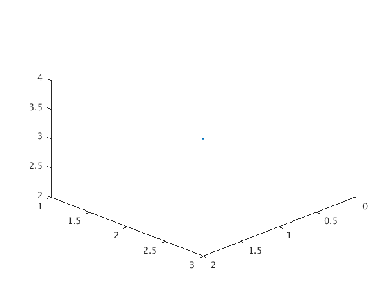
And here are two points
plot3(1,2,3,'o',-1,2,5,'o')
view([10 10 10])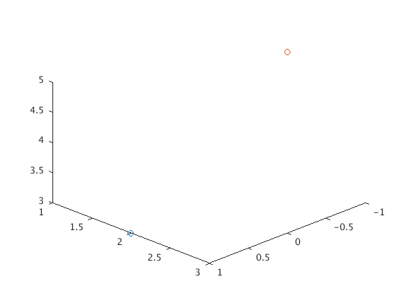
Note the 'o' tells Matlab to draw circles for points. Also note the view command there. Matlab has an annoying habit of viewing the axes from a nonstandard angle. The view([10 10 10]) command puts our point-of-view at the point $(10, 10, 10)$ so we look down at the origin as we’re used to in class.
Important observation! On the figure window there is a little rotation button which allows you to drag the picture around and look at it from different angles. Very useful and fun too! I can’t demonstrate in a fixed html document though.
Plotting Curves
Okay now, let’s plot some curves! We’ll use the 3D command fplot3. In class we sketched a helix with $\mathbf{r}(t) = \cos(t)\mathbf{i} + \sin(t)\mathbf{j} + t\mathbf{k}$.
fplot3(cos(t),sin(t),t,[0,6*pi])
view([10 10 10])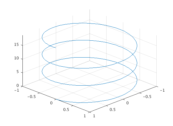
Here’s a different thing - it’s a circle but the z-value is oscillating as well, five times around the circle:
fplot3(cos(t),sin(t),sin(5*t),[0,2*pi])
view([10 10 10])
If you have a vector-valued function defined already and wish to fplot3 it then you need to give it the component functions. You can do this like:
r=[t,-t,t^2];
fplot3(r(1),r(2),r(3),[-1,1])
view([10 10 10])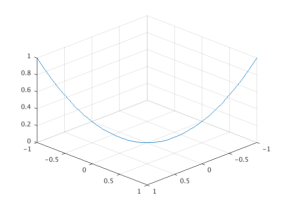
Plotting Vectors
Here’s a vector in 3D. The first three coordinates are the anchor point and the last three are the vector. So this is the vector $3\mathbf{i} + 4\mathbf{j} − 2\mathbf{k}$ anchored at $(1, 2, 3)$.
quiver3(1,2,3,3,4,-2)
view([10 10 10])
daspect([1 1 1])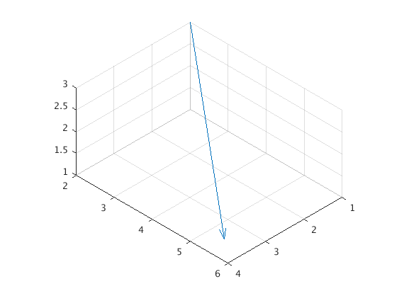
This last command daspect sets the aspect ratio so that all the axes are scaled the same. I have no idea why Matlab doesn’t do this by default but grumble grumble grumble.
Plotting Planes
Just to close out let’s draw some planes. Matlab has a great command patch which draws a polygon. To use this to draw a plane we need to give it several points on the plane. It’s a bit awkward - we need to give the points in order around the plane in either direction and we need to give it the $x$-coordinates together and the $y$-coordinates together. There’s a slick way to do the second part but for the first part we just need to choose the points carefully, following around the part of the plane we want to plot. Here are some examples:
For the plane $x + 2y + 3z = 12$ we’ve seen that we can get a good picture using the intercepts $(12, 0, 0)$ and $(0, 6, 0)$ and $(0, 0, 4)$. The order we take them in doesn’t matter since any order will either be counterclockwise or clockwise. To draw this with patch we do:
figure
points = [12 0 0;0 6 0;0 0 4];
patch(points(1,:),points(2,:),points(3,:),[0.95 0.95 0.95]);
view([10 10 10])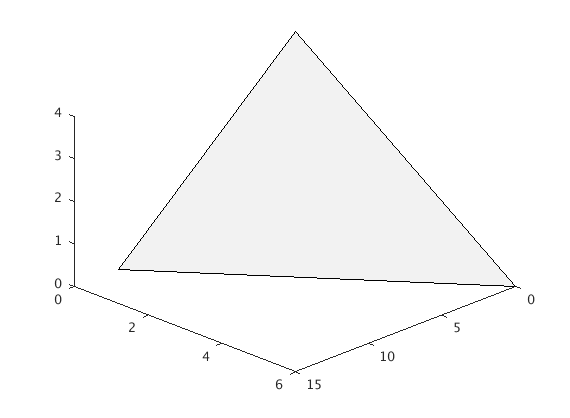
For the plane $2x+ 4y = 20$ we've seen that the way to approach this is to draw the line $2x+ 4y = 20$ in the $xy$-plane and then extend upwards. The $x$ and $y$-intercepts are $(10, 0, 0)$ and $(0, 5, 0)$ so we’ll plot those along with $(10, 0, 10)$ and $(0, 5, 10)$. Note that the order we've chosen goes around the piece of the plane.
figure
points = [10 0 0;0 5 0;0 5 10;10 0 10];
patch(points(:,1),points(:,2),points(:,3),[0.95 0.95 0.95]);
view([10 10 10])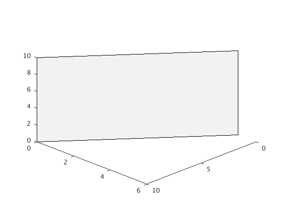
 - Sam Punshon-Smith 2017