MATLAB Project 3 Due: W 11/15

The following material has been adapted and copied with permission from material created by Justin Wyss-Gallifent.

The basic format of this guide is the same as the first two. The project involves creating a script m-file and put the tasks in order into that file, then publishing that file using MATLAB's publish to HTML feature and printing the resulting document. You should separate each task into cells with the title of the task preceded by a %%.

---

Multiple Integrals

Since MATLAB does integrals so well this is easy, we just nest the integrals. For example consider the following. Read it carefully from the innermost int outwards. Remember that when we do int(f,x,a,b) we integrate f with respect to x from a to b. Here a and b may also contain other variables.

For example if we wanted to do $$\int_{-1}^2 \int_0^{2x}\int_{x+y}^x x^2y + z \mathrm{d}z\mathrm{d}y\mathrm{d}x$$

syms x y z
int(int(int(x^2*y+z,z,x+y,x),y,0,2*x),x,-1,2)

ans =

-81/2

Here's the integral $$\int_0^{2\pi}\int_{0}^{\pi/4}\int_{2\sec\phi}^5\rho^4\sin\phi\mathrm{d}\rho\mathrm{d}\phi\mathrm{d}\theta$$

syms theta rho phi
int(int(int(rho^4*sin(phi),2*sec(phi),5),0,pi/4),0,2*pi)

ans =

-(pi*(3125*2^(1/2) - 6202))/5

Plotting Surfaces

In Section 14.9 we learn how to parameterize surfaces as vector-valued functions of two variables. This is perfect for the fsurf command.

Here is the part of the cone $z= \sqrt{x^2+y^2}$ with $-3\leq x \leq 1$ and $-2 \leq y \leq 1$.

clear all;
syms x y;
rbar = [x,y,sqrt(x^2 + y^2)];
fsurf(rbar(1),rbar(2),rbar(3),[-3,1,-2,1])
view([10 10 10])
axis equal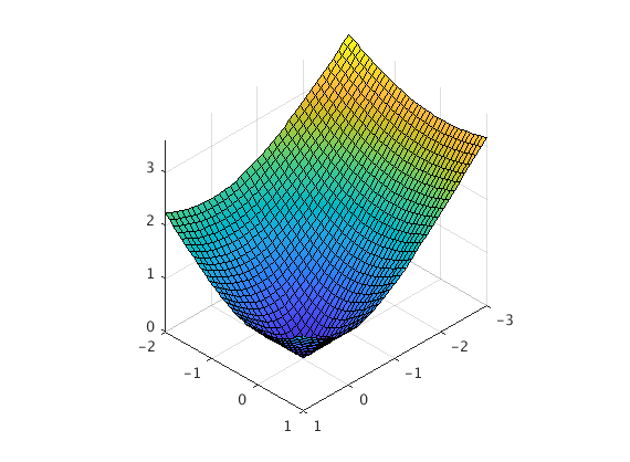

A few things to note:

• I am setting view([10 10 10]) which puts the viewpoint in the first octant looking in.
• I have set axis equal which ensures that all three axis are proportionally scaled, making the pictures look better.
• We have to give the fsurf the three components separately. We do this by giving it r(1), r(2) and r(3).
• The restrictions are in alphabetical order so for x, y and z it works as expected.

Here is the portion of the sphere of radius $2$ inside the cone $\phi = \pi/3$ done using $r$ and $\phi$. The restriction on phi must come first for alphabetical reasons.

clear all;
syms phi t;
rbar = [2*sin(phi)*cos(t),2*sin(phi)*sin(t),2*cos(phi)];
fsurf(rbar(1),rbar(2),rbar(3),[0,pi/3,0,2*pi])
view([10 10 10])
axis equal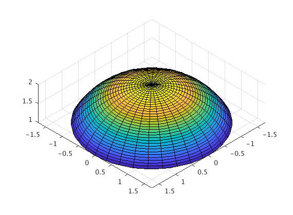

Here is something really cool, a spiral!

clear all;
syms t z;
rbar = [t*cos(t),t*sin(t),z];
fsurf(rbar(1),rbar(2),rbar(3),[0,6*pi,0,10])
view([10 10 10])
axis equal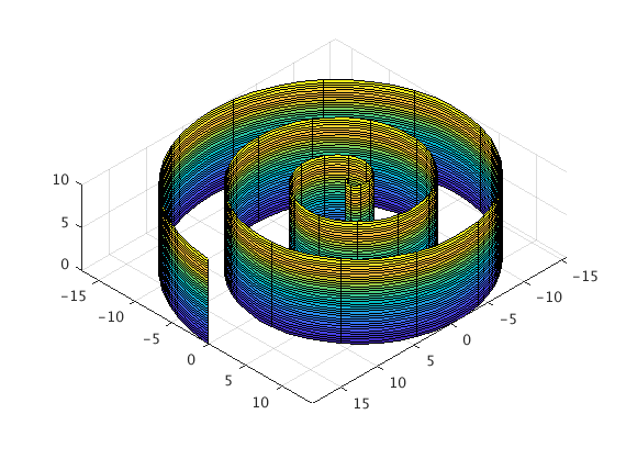

---

Vector Fields

Matlab can plot vector fields using the quiver command, which basically draws a bunch of arrows. This is not completely obvious though. First we have to set up a grid of points for which to plot arrows. In other words we have to tell it for which x and y to actually draw the vector field.

Suppose we want our grid to have x going from -5 to 5 in steps of 1 and the same for y. We first do the following:

clear all;
[x,y] = meshgrid(-5:1:5,-5:1:5);

Now suppose we wish to plot the vector field $\mathbf{F}(x,y) = \frac{y}{5}\mathbf{i} - \frac{x}{5}\mathbf{j}$. To do this we type

quiver(x,y,y/5,-x/5,0);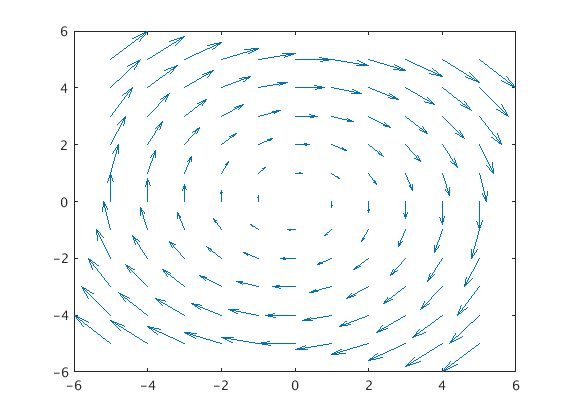

A window will pop up with the vector field on it. The 0 at the end just ensures that Matlab does not do any tricky rescaling of the vectors, something it usually does to make things fit nicely.

Just so you know the first two entries x, y indicate that vectors should be place at x,y. The second two entries form the vector itself.

A note of caution. Suppose we want the vector field $\mathbf{F}(x,y)=\frac{y}{5}\mathbf{i}-\frac{x}{y}\mathbf{j}$. Since x and y are collections of numbers, to divide them we cannot use /, we must use ./ instead. This is a Matlab quirk since we are not working with individual numbers. Thus we would need:

quiver(x,y,y./5,-x./y,0)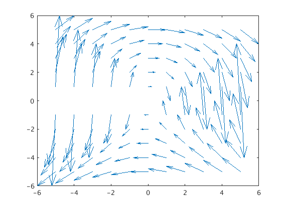

Note that this is a pretty ugly vector field. Try it!

---

Vector Fields in 3D

For 3D vector fields we use quiver3. Here is an example. It's the only one we'll do because they can be pretty overwhelming.

[x,y,z] = meshgrid(-5:2:5,-5:2:5,-5:2:5);
quiver3(x,y,z,-y./sqrt(x.^2+y.^2),x./sqrt(x.^2+y.^2),z./5,0)
view([10 10 10])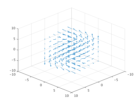

---

Line Integrals of Functions

Line integrals of functions are really easy - we just tell Matlab exactly what to do, step by step. For example here is Example 1 from page 1006 of the text.

clear
syms t x y z;
rbar = [t,-3*t,2*t];
f = x+y^2-2*z;
mylength = @(u) sqrt(u*transpose(u));
mag = simplify(mylength(diff(rbar,t)));
sub = subs(f,[x,y,z],rbar);
int(sub*mag,t,0,1)

ans =

(3*14^(1/2))/2

Read this carefully to see how it works! Especially note the line mylength=... which creates a new length function for vectors. The Matlab norm command only works on numerical vectors and not on vectors with variables in them. Our new mylength function will do the job. Even if you don’t understand it for now just use it - all it does is finds the norm of a vector even if that vector contains variables.

---

Line Integrals of Vector Fields

Just like line integrals of functions these are easy, we just tell Matlab exactly what we want it to do. Here’s Example 6 from page 1011 of the text. Again read carefully and understand!

clear all
syms t x y z;
rbar = [t,t^2,t^3];
F = [x*y,3*z*x,-5*x^2*y*z];
sub = subs(F,[x,y,z],rbar);
int(dot(sub,diff(rbar,t)),0,1)

ans =

-1/4